Price and Output Under Oligopoly

In order to explain kinked demand curve and price rigid­ity, fol­low­ing assump­tions are made: (i) There are two firms namely A and B. (ii) Prod­uct of both the firms is homo­ge­neous.

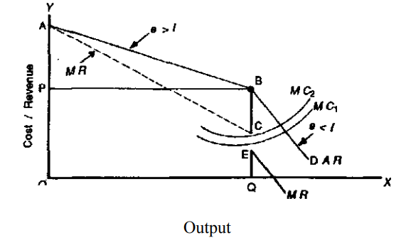
(iii) There is a par­tic­u­lar price pre­vail­ing in the mar­ket, assumed to be OP as shown in the fig­ure. The demand curve-AD is kinked at B with its two seg­ments. The seg­ment AB is rel­a­tively more elas­tic and the seg­ment BD is rel­a­tively less elas­tic. Since the demand curve (AR)-AD is dis­con­tin­u­ous, so the cor­re­spond­ing MR curve is also not con­tin­u­ous. The MR curve's seg­ment AC cor­re­sponds to AR curve's seg­ment AB. The MR curve's seg­ment start­ing from E cor­re­sponds to BD seg­ment of the AR curve. Let us assume that the firm A raises the price above the pre­vail­ing price OP. Now the firm B will not raise the price. As a result, the demand for A's pro­duc­tion will decline con­sid­er­ably. This is why the AB seg­ment of the demand curve is more elas­tic. Since firm B has not fol­lowed the price rise, firm A will bring its price back down. Hence the price is rigid at OP.

Let us now assume that the firm A reduces the price below pre­vail­ing price OP. Now firm B reacts by reduc­ing the price so that firm A does not take away the whole mar­ket. As a result of this, the firm A will not have any increase in the demand for its prod­uct. Hence, BD seg­ment of the demand curve-AD is rel­a­tively less elas­tic. As firm A has gained noth­ing by cut­ting its price, it will return to the pre­vail­ing price OP. Hence, the price is rigid at OP.

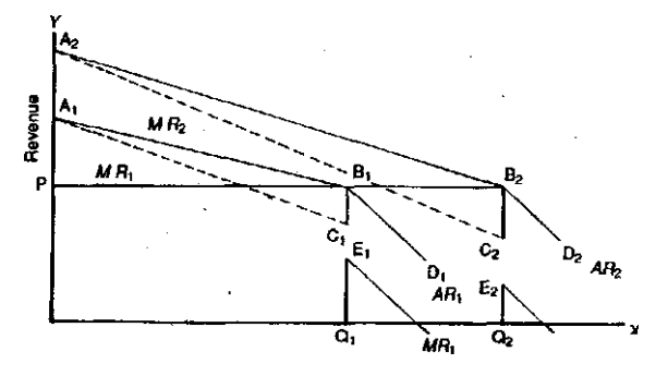
The price rigid­ity or stick­i­ness is also shown by the fact that a shift in the MC curve also does not affect the price. It is evi­dent from the fig­ure that despite shift in MC curve from MC1 to MC2 the price remains rigid at the level of OP. Note that in the kinked demand model the price is not pinned down by MC = MR alone, because the MC curve passes through the gap CE in the MR curve. The price also remains rigid despite shift in the demand curve. In the fig­ure, the demand curve (AR) – A1D1 shifts to the right to A2D2, but the price is rigid at OP level.

In short, Paul Sweezy has empha­sised the price rigid­ity as the basic fea­ture of the non-col­lu­sive oli­gop­oly. Kinked demand curve is the log­i­cal deduc­tion from price rigid­ity.

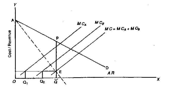
The term 'col­lu­sion' implies 'to play togeth­er'. The oli­gop­o­lis­tic firms arrive at a for­mal agree­ment about price-out­put instead of com­pet­ing with each other. The com­pet­ing firms form a 'cartel'. The 'cartel' is a com­mon sales agency formed to elim­i­nate com­pe­ti­tion and fix such a price and quan­tity of out­put that will max­imise prof­its of the mem­ber firms. The car­tel deter­mines the price-out­put for whole of the indus­try as well as for each mem­ber firm. In other words, the car­tel admin­is­tra­tion deter­mines the equi­lib­rium total out­put as well as the equi­lib­rium quan­tity of out­put for each mem­ber firm. The price-out­put deter­mi­na­tion by the car­tel admin­is­tra­tion can be explained on the basis of the fol­low­ing assump­tions: (i) It is assumed that there are two firms namely A and B. These firms form a car­tel. (ii) The prod­ucts of firms A and B are homo­ge­neous. (iii) The costs of pro­duc­tion of firms A and B are dif­fer­ent. (iv) The car­tel deter­mines such price-out­put com­bi­na­tion which ensures max­i­mum prof­its for whole of the oli­gop­o­lis­tic indus­try. The car­tel esti­mates the total demand for the indus­try's prod­uct it is sig­ni­fied by the curve-AD in the fig­ure. The mar­ginal rev­enue curve - MR in the dia­gram shows cartel's rev­enue from the sale of the addi­tional quan­tity of out­put. Car­tel’s MC curve is the hor­i­zon­tal sum­ma­tion of the mar­ginal cost curves of the firms A and B. The equi­lib­rium of the oli­gop­o­lis­tic indus­try is denoted by E, where MC = MR. The equi­lib­rium price is QP and the equi­lib­rium total out­put is OQ.

Hav­ing decided that total out­put will be OQ, the car­tel allots the out­put quota to each mem­ber firm so that the mar­ginal cost of each firm is the same. This can be deter­mined by draw­ing a hor­i­zon­tal straight line from E towards the Y-axis. The firm A pro­duces OQ1 out­put and the firm B pro­duces OQ2 out­put. The total out­put OQ is equal to OQ1 + OQ2. In short, price QP and out­put OQ ensure joint prof­its to the mem­bers of the car­tel or indus­try.

Accord­ing to price lead­er­ship model of oli­gop­oly, the leader firm in the mar­ket deter­mines the price of the prod­uct. The firm which acts as the leader firm is one which is either a low-cost firm, a dom­i­nant firm or an expe­ri­enced and respected firm. Accord­ingly, the most com­mon types of lead­er­ship are:

(i) Price lead­er­ship by a low-cost firm,

(ii) Price lead­er­ship by a large (dom­i­nant) firm,

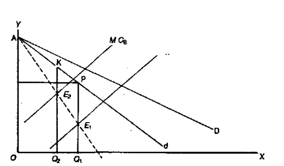
(iii) Baro­met­ric price lead­er­ship (expe­ri­enced and respected firm). The leader firm deter­mines the price by using the mar­gin­al­is­tic rule of MC = MR. The Leader firm is a price-maker, and the other firms are price-tak­ers. The price-taker firms max­imise their prof­its by adopt­ing the price fixed by the leader firm. Price Lead­er­ship by a Low-cost Firm: The price-out­put deter­mi­na­tion under this model is based on the fol­low­ing assump­tions: (i) It is assumed that there are two firms A and B. (ii) The prod­uct pro­duced by the two firms is homo­ge­neous, (iii) The firm A being the low-cost firm acts as a leader firm, (iv) Each of the two firms has an equal share in the total mar­ket.

In the fig­ure, AD is the mar­ket demand curve. Each of the two firms has a demand curve Ad. MR is the mar­ginal rev­enue curve of each firm. MCA is the mar­ginal cost curve of firm A and MCB is the mar­ginal cost curve of firms B. MCA lies below MCB because we are assum­ing that firm A is a low-cost firm act­ing as a Leader firm. The Leader firm A is in equi­lib­rium at E1 where MCA = MR. The firm A max­imises prof­its by sell­ing out­put OQ1 and set­ting price Q1P. The firm B can max­imise prof­its by pro­duc­ing OQ2 out­put and sell­ing it at Q2K price as these cor­re­spond to its equi­lib­rium at E2 where MCB = MR. Since the firm B has to com­pete with the low-cost firm A (Leader firm), there­fore it will be defeated in the price war if it fixes up Q1K price which is higher than the Q1P price of the leader firm A. Hence, the firm B will be com­pelled to fol­low the Leader firm A. The firm B will charge the price Q1P as set by firm A. It will also pro­duce OQ1 out­put which is the equi­lib­rium out­put of the Leader firm A. To con­clude, Q1P price will pre­vail in the mar­ket and total out­put will be twice of OQ1.

Com­mon ques­tions#

Why are prices mostly sta­ble in non-col­lu­sive oli­gop­o­lies?#

In a non-col­lu­sive oli­gop­oly there are only a few large firms, and chang­ing prices does not ben­e­fit any of them. When one firm raises its price, other firms main­tain their price level. As such, con­sumers buy goods from other firms at a lower price. Like­wise, when one firm low­ers its price, other firms also decrease their prices so that they do not lose cus­tomers.

Oli­gop­o­lis­tic mar­kets, thus, give rise to kinked demand curves. At higher prices, the demand curve is highly elas­tic. And at lower prices, the demand curve is rel­a­tively inelas­tic. The kink is present at the inter­sec­tion of the two demand curves.

Why are there only a few firms in an oli­gop­oly?#

Firms need to invest huge sums to enter and sur­vive, and to cope with swings in demand, sup­ply and mar­gins. Because any change in pol­icy or pric­ing by one firm changes the game for all the oth­ers, each must stay alert and a step ahead. So there are few com­peti­tors, but the com­pe­ti­tion among them is fierce.