Price and Output Under Monopoly

Demand and Rev­enue under Monop­oly#

In monop­oly, there is only one pro­ducer of a prod­uct, who influ­ences the price of the prod­uct by chang­ing its sup­ply. The pro­ducer under monop­oly is called monop­o­list. If the monop­o­list wants to sell more, he/she can reduce the price of a prod­uct. On the other hand, if he/she is will­ing to sell less, he/she can increase the price.

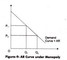
Under monop­oly there is no dif­fer­ence between the firm and the indus­try. So the demand curve of the firm is the demand curve of the entire indus­try. The demand curve of the monop­o­list is Aver­age Rev­enue (AR), which slopes down­ward.

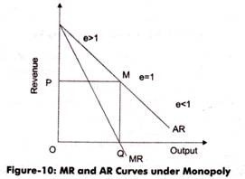
In the fig­ure, it can be seen that more quan­tity (OQ2) can only be sold at lower price (OP2). Under monop­oly, the slope of AR curve is down­ward, which implies that if the high prices are set by the monop­o­list, the demand will fall. In addi­tion, in monop­oly, AR curve and Mar­ginal Rev­enue (MR) curve are dif­fer­ent from each other. How­ever, both of them slope down­ward.

What the down­ward-slop­ing AR and MR curves show#

i. When MR is greater than AR, the AR rises.

ii. When MR is equal to AR, AR remains con­stant.

iii. When MR is less than AR, AR falls.

Here AR is the price of the prod­uct. Since AR falls under monop­oly, MR is less than AR.

AR and MR curves under monop­oly#

In the fig­ure, the MR curve lies below the AR curve because AR is falling.

A numer­i­cal cal­cu­la­tion of AR and MR under monop­oly#

As shown in the table, AR is equal to price. MR is less than AR and falls twice as fast. For instance, when out­put rises from one unit to two, MR falls by Rs. 2, whereas AR falls by Re. 1.

Monop­oly Equi­lib­rium#

Under monop­oly a sin­gle firm is the whole indus­try, so there is no need to analyse the equi­lib­rium of the firm and of the indus­try sep­a­rately. Like a pro­ducer in per­fect com­pe­ti­tion, the monop­o­list aims to earn max­i­mum profit.

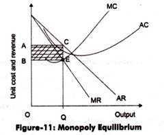
As in per­fect com­pe­ti­tion, equi­lib­rium is reached where profit is max­i­mum, that is, where MR = MC. The monop­o­list will go on pro­duc­ing addi­tional units as long as MR is greater than mar­ginal cost (MC).

In the fig­ure, if out­put is increased beyond OQ, MR will be less than MC. Thus, if addi­tional units are pro­duced, the orga­ni­za­tion will incur loss. At equi­lib­rium point, total prof­its earned are equal to shaded area ABEC. E is the equi­lib­rium point at which MR=MC with quan­tity as OQ.

Under monop­oly, price is related to MC as fol­lows:

Price = AR

MR= AR [(e-1)/e]

e = Price elas­tic­ity of demand

As in equi­lib­rium MR=MC

MC = AR [(e-1)/e]

Deter­min­ing Price and Out­put under Monop­oly#

Sup­pose the monop­o­list's demand func­tion is Q = 100 – 0.1P

so the price func­tion is P = 1000 – 10Q

and the cost func­tion is TC = 100 + 40Q + Q²

Max­i­mum profit is achieved where MR=MC

To find MR, TR is derived.

TR = (1000 – 10Q) Q = 1000Q – 10Q²

MR = ∆TR/∆Q= 1000 – 20Q

MC = ∆TC/∆Q = 40 + 2Q

MR = MC

1000 – 20Q = 40 + 2Q

960 = 22Q, so Q = 43.64 (about 44), the profit-max­imis­ing out­put

Profit-max­imis­ing price = 1000 – 10 × 44 = 560

Total max­i­mum profit = TR – TC = (1000Q – 10Q²) – (100 + 40Q + Q²)

At Q = 44

Total max­i­mum profit = 24,640 – 3,796 = Rs. 20,844

Monop­oly Equi­lib­rium in Case of Zero Mar­ginal Cost#

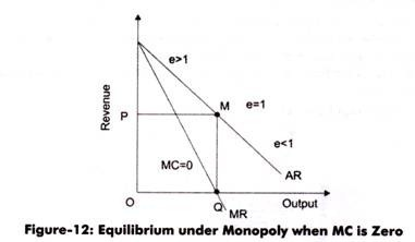
In cer­tain sit­u­a­tions MC may be zero, for exam­ple when the cost of pro­duc­ing spring water is taken as zero. The monop­o­list still sets a price that earns a profit.

In the fig­ure, AR is the aver­age rev­enue curve and MR is the mar­ginal rev­enue curve. Since MC is zero, the con­di­tion MR = MC becomes MR = 0. As the fig­ure shows, equi­lib­rium is reached where MR equals zero, that is at out­put OQ and price P. We can see that point M is the mid-point of AR curve, where elas­tic­ity of demand is unity. There­fore, when MC = 0, the equi­lib­rium of the monop­o­list is estab­lished at the out­put (OQ) where elas­tic­ity of demand is unity.

Short-Run and Long-Run View under Monop­oly#

Till now, we have dis­cussed monop­oly equi­lib­rium with­out tak­ing into con­sid­er­a­tion the short-run and long- run period. This is because the short-run and long-run analy­ses of monop­oly do not dif­fer much.

In the short run, the monop­o­list should make sure that the price should not go below Aver­age Vari­able Cost (AVC). The equi­lib­rium under monop­oly in long-run is same as in short-run. How­ever, in long-run, the monop­o­list can expand the size of its plants accord­ing to demand. The adjust­ment is done to make MR equal to the long run MC.

In the long-run, under per­fect com­pe­ti­tion, the equi­lib­rium posi­tion is attained by entry or exit of the orga­ni­za­tions. In monop­oly, the entry of new orga­ni­za­tions is restricted.

The monop­o­list may hold some patents or copy­right that lim­its the entry of other play­ers in the mar­ket. When a monop­o­list incurs losses, he/she may exit the busi­ness. On the other hand, if prof­its are earned, then he/she may increase the plant size to gain more profit.