In the short run some inputs are fixed. Here is how fixed, variable, marginal and average costs are defined, and how MC = W/MPL and AVC = W/APL link cost to productivity.
In the short run, some of the firm’s inputs to production are fixed, yet others can be varied to change the rate of output.
The total cost of production has two components: the fixed cost, FC, which is borne by the firm, whatever level of output it produces, and the variable cost, VC, which varies with the level of output. Fixed costs may include expenditures for plant maintenance, insurance, a minimal number of employees, etc., these costs remain unchanged no matter how much the firm produces.
Variable costs include expenditure on wages, salaries and raw materials, and these costs increase as output increases.
Total Cost = Total Fixed Cost + Total Variable Costs.
Fixed costs can be controlled in the long run but do not vary with the level of output in the short-run. They must be paid even if there is no output. A firm can only forgo its outlays on fixed costs when it decides to go out of business.
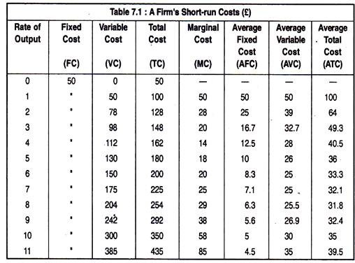
Since fixed costs must be paid whatever the output, the manager deciding how much to produce needs to know above all how variable costs rise with output. For this we need some further cost measures, which we explain with an example typical of many firms, and then relate to the production process. The table below describes a firm with a fixed cost of £50. Variable cost increases with output, as does the total cost. The total cost is the sum of fixed cost in column (1) and the variable cost in column (2). From the cost figures given in columns (1) and (2), several additional cost variables can be defined.
Average cost is the cost per unit of output. There are three types of average cost: average fixed cost, average variable cost and average total cost. Average fixed cost (AFC) is the total fixed cost (column 1) divided by the level of output, TFC/Q. Because fixed cost is constant, average fixed cost declines as the rate of output increases.
Marginal cost (MC), also called incremental cost, is the increase in cost that results from producing one extra unit of output. Since FC does not change as the firm’s level of output changes, MC is just the increase in variable cost that results from an extra unit of output.
We can thus write MC as MC = ΔVC/ΔQ. MC tells us how much it will cost to expand the firm’s output by one unit. In the table, MC is calculated from either the VC (column 2) or the total cost (column 3).
AVC is the total variable cost divided by the level of output, TVC/Q. Finally, average total cost (ATC) is the total cost divided by the level of output, TC/Q. The average total cost tells us the per-unit cost of production. By comparing the ATC to the price of the product, we can determine whether production is profitable.
The table shows that variable and total costs increase with output. The rate at which these costs increase depends on the nature of the production process, and, in particular, on the extent to which production involves diminishing returns to variable factors.
Let us look at the relationship between production and cost in more detail by concentrating on the costs of a firm that can hire as much labour as it wishes at a fixed wage W.
We know that marginal cost (MC) is the change in variable cost for a one-unit change in output (i.e., ΔVC/ΔQ). But the extra variable cost is the per-unit cost of the extra labour, W, times the amount of extra labour, ΔL. It follows that MC = ΔVC/ΔQ = WΔL/ΔQ.
The marginal product of labour MPL is the change in output resulting from a one-unit change in labour input, or ΔQ/ΔL. Thus, the extra labour needed to obtain an extra unit of output is ΔL/ΔQ = 1/MPL. As a result, MC = W/MPL ………….(1).
Equation (1) states that, in the short-run, MC = price of the input that is being varied divided by the MP. When MP is high, the labour requirement is low, as is the MC. More generally, whenever the MPL decreases, the MC of production increases, and vice versa. The effect of the presence of diminishing returns in the production process can also be seen by looking at the MC figures in the table.
The MC of additional output is high at first because the first few inputs to production are not likely to raise output much in a large plant with a lot of equipment. However, as the inputs become more productive, the MC decreases substantially. Finally, MC increases again for relatively high level of output, owing to the effect of diminishing returns.
The law of diminishing returns also creates a direct link between the APL and the AVC of production. AVC is equal to the variable cost per unit of output, or VC/Q. When L units of labour are used in the production process, the variable cost is WL. Thus, AVC = WL/Q. The average product of labour, APL, is output per unit of labour, Q/L. As a consequence, AVC = W/APL……………….. (2).
Since the wage rate is fixed for the firm, there is an inverse relationship between AVC and the AP of labour. A lower average product of labour means that a large amount of labour is needed to produce the firm’s output, which leads to a higher AVC. A high AP of labour means that the labour required for production is low, as is the AVC.
We have seen that, with both MC and AVC, there is a direct link between factor productivity and the costs of production. Marginal and average products tell us about the relationship between inputs and output. The corresponding cost measures tell us about the budgetary implications of the production function.