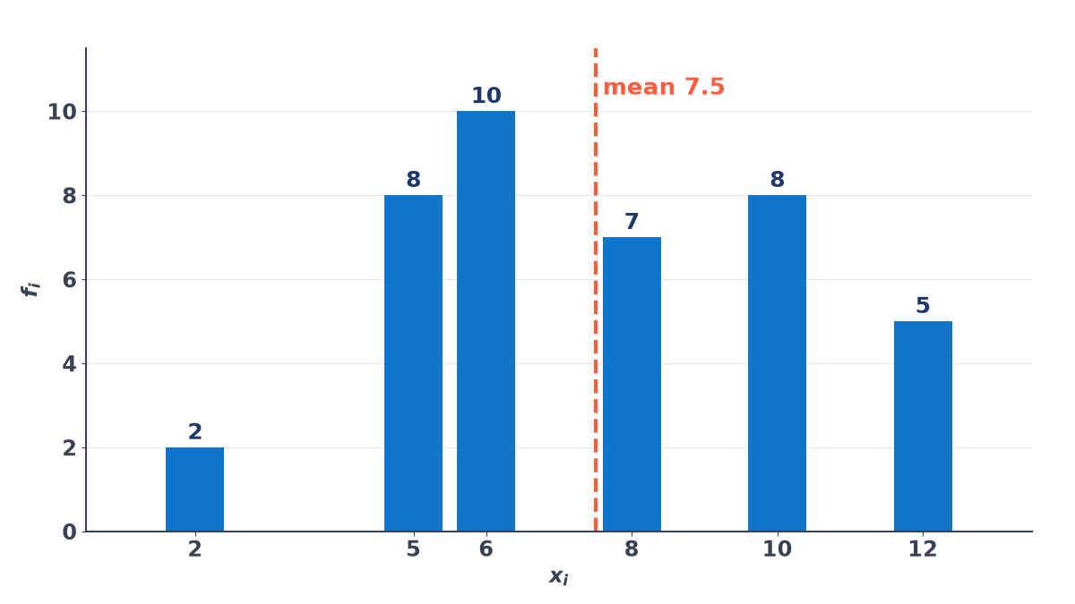
Two batsmen both average 40 runs, yet one is steady match after match while the other swings between ducks and centuries. Which one would you pick for a tight chase? The average cannot tell you; it hides exactly this difference. A measure of dispersion brings it out. We will start with the range, then meet the mean deviation, both about the mean and about the median, and compute it for raw data, discrete frequency tables and grouped data.
The mean deviation about a central value a is simply the average distance of the observations from a:
MD(a)=n1∑∣xi−a∣or, with frequencies,N1∑fi∣xi−a∣.
For a we usually take the mean xˉ or the median M. (Of all choices, the median gives the smallest possible mean deviation.)
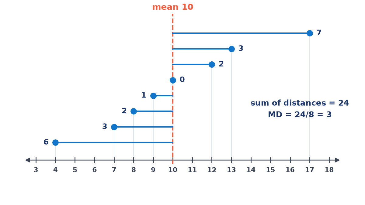
Example 1. Data 4,7,8,9,10,12,13,17: xˉ=880=10. The deviations are 6,3,2,1,0,2,3,7, which add up to 24, so MD(xˉ)=3.
Example 1: the average distance from the mean 10 is 3
Example 2. Data 13,17,16,14,11,13,10,16,11,18,12,17. Sort them first; the two middle values are 13 and 14, so M=13.5. The deviations add up to 28, so MD(M)=1228=2.33.
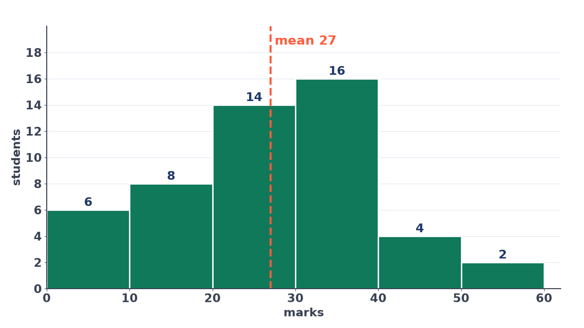
With grouped data, use the class midpoints as the xi. For the median, M=l+f2N−C×h, where l is the lower limit of the median class, C the cumulative frequency before it, f its frequency and h the class width.
Where it falls short. Absolute values are clumsy to handle in algebra, and the mean deviation treats a large deviation no more seriously than its size alone. That is why, in the next lesson, we will usually prefer the variance.