EOQ in Operations Management (Economic Order Quantity)

Eco­nomic Order Quan­tity (EOQ) is the quan­tity of an item that should be ordered each time so that the total of annual order­ing cost and annual car­ry­ing (hold­ing) cost is as low as pos­si­ble. Order too often and order­ing cost climbs; order too much at once and stor­age cost climbs. EOQ is the order size that bal­ances the two.

It mat­ters because every busi­ness that buys stock repeat­edly must answer "how much should we order each time?" Choos­ing the fig­ure at ran­dom wastes money through too many orders or through blocked cap­i­tal and crowded stores. The EOQ model, first pub­lished by Ford W. Har­ris in 1913, remains the foun­da­tion of inven­tory the­ory and a stan­dard exam topic in BBA, B.Com and MBA courses.

Mean­ing of EOQ in sim­ple words

Imag­ine a gro­cery store buy­ing rice. If it orders every two days, trans­port, paper­work and order­ing effort pile up. If it buys six months' rice at once, stor­age cost, spoilage risk and blocked money rise. The shop wants one order size that is nei­ther too small nor too big. That best quan­tity is the EOQ. A col­lege sta­tionery store sell­ing pens all year faces the same choice: very small repeated orders increase effort, very large orders fill the shelves and block money.

Why EOQ is impor­tant

With­out a rule, stock cost increases, space is wasted, too many orders are placed, cap­i­tal is blocked and con­trol becomes inef­fi­cient. EOQ helps a busi­ness:

• reduce total inven­tory cost;
• make order­ing sys­tem­atic and sci­en­tific rather than guess­work;
• bal­ance order­ing cost and car­ry­ing cost;
• avoid both over-order­ing and too-fre­quent order­ing;
• plan pur­chas­ing fre­quency and stock lev­els.

Main objec­tive

The objec­tive is to find the most eco­nom­i­cal order size, one at which order­ing cost is not too high, car­ry­ing cost is not too high, and their total is min­i­mum. EOQ is a cost-min­imis­ing inven­tory tool.

The two costs EOQ bal­ances

Order­ing cost

The cost of plac­ing one order: paper­work, com­mu­ni­ca­tion, fol­low-up, trans­port arrange­ment, and receiv­ing and inspec­tion. It is treated as fixed per order, so annual order­ing cost rises with the num­ber of orders.

Car­ry­ing or hold­ing cost

The expense of stor­ing inven­tory for a spec­i­fied period: ware­house rent, insur­ance, inter­est on blocked cap­i­tal, spoilage, dete­ri­o­ra­tion, obso­les­cence and secu­rity. Annual car­ry­ing cost rises with aver­age stock. It is often stated as a per­cent­age of unit price.

The trade-off

The basic model does not con­sider changes in pur­chase price; the price is assumed con­stant, so it does not affect the choice of order size. Quan­tity dis­counts are han­dled by an exten­sion dis­cussed later.

The EOQ for­mula

Let $D$ be annual demand (annual usage) in units, $S$ the order­ing cost per order, $H$ the hold­ing cost per unit per year and $Q$ the order quan­tity.

With steady use, stock falls from $Q$ to zero in a straight line and is then replen­ished, so the aver­age inven­tory is $\displaystyle \frac{Q}{2}$. The num­ber of orders per year is $\displaystyle \frac{D}{Q}$. There­fore:

$$\displaystyle \text{Annual ordering cost} = \frac{D}{Q} \times S, \qquad \text{Annual carrying cost} = \frac{Q}{2} \times H$$

$$\displaystyle TC = \frac{D}{Q}S + \frac{Q}{2}H$$

Total cost is low­est where the two parts are equal (equiv­a­lently, where the deriv­a­tive of $TC$ with respect to $Q$ is zero):

$$\displaystyle \frac{D}{Q}S = \frac{Q}{2}H \quad \Rightarrow \quad Q^2 = \frac{2DS}{H}$$

$$\displaystyle EOQ = \sqrt{\frac{2DS}{H}}$$

If car­ry­ing cost is given as a per­cent­age $i$ of unit price $C$, then $H = iC$ and $\displaystyle EOQ = \sqrt{\frac{2DS}{iC}}$. Annual usage is one of the essen­tial com­po­nents of the for­mula, and $D$ and $H$ must use the same time period.

How each vari­able affects EOQ

• Higher annual demand raises EOQ (but only by the square root: four times the demand gives twice the EOQ).
• Higher order­ing cost raises EOQ: order larger quan­ti­ties less often.
• Higher hold­ing cost low­ers EOQ: keep less stock.

Worked exam­ple: cal­cu­lat­ing EOQ

Sup­pose a man­u­fac­turer uses 10,000 units of a com­po­nent a year. Order­ing cost is ₹100 per order, and hold­ing cost is ₹5 per unit per year (10% of a ₹50 unit price). The firm works 250 days a year, and sup­plier lead time is 5 days.

Step 1: EOQ

$$\displaystyle EOQ = \sqrt{\frac{2 \times 10{,}000 \times 100}{5}} = \sqrt{\frac{20{,}00{,}000}{5}} = \sqrt{4{,}00{,}000} \approx 632.46 \approx 632 \text{ units}$$

Step 2: num­ber of orders per year

$$\displaystyle N = \frac{D}{EOQ} = \frac{10{,}000}{632.46} \approx 15.81 \text{ orders (about 16)}$$

Step 3: annual costs at EOQ

$$\text{Ordering cost} = 15.81 \times 100 = \text{ ext{₹}}1{,}581.14$$

$$\displaystyle \text{Carrying cost} = \frac{632.46}{2} \times 5 = 316.23 \times 5 = \text{ ext{₹}}1{,}581.14$$

$$TC = 1{,}581.14 + 1{,}581.14 = \text{ ext{₹}}3{,}162.28$$

The two costs are equal at EOQ, as the deriva­tion pre­dicts.

Step 4: time between orders

$$\displaystyle T = \frac{\text{Working days}}{N} = \frac{250}{15.81} \approx 15.8 \text{ days}$$

Step 5: reorder point

Daily demand is $\displaystyle \frac{10{,}000}{250} = 40$ units. With a 5-day lead time and no safety stock:

$$ROP = 40 \times 5 = 200 \text{ units}$$

So when stock falls to 200 units, an order for 632 units is placed.

Step 6: check­ing other order sizes

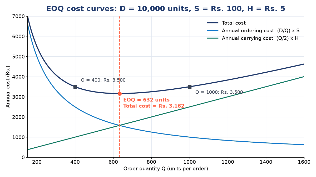
This flat bot­tom is an impor­tant prac­ti­cal point: EOQ is robust. Round­ing the answer to a con­ve­nient pack size, or small errors in esti­mat­ing $S$ or $H$, change total cost only slightly. Here, mov­ing 37% below EOQ raises cost by $\displaystyle \frac{3{,}500 - 3{,}162.28}{3{,}162.28} \times 100 \approx 10.7\%$.

A sec­ond quick exam­ple

If annual demand is 12,000 units and EOQ is 600 units, the firm places $\displaystyle \frac{12{,}000}{600} = 20$ orders a year. Work­ing 300 days, it orders every $\displaystyle \frac{300}{20} = 15$ days, and aver­age inven­tory is $\displaystyle \frac{600}{2} = 300$ units.

Graph­i­cal under­stand­ing of EOQ

Order­ing cost curve

As order quan­tity increases, annual order­ing cost falls because fewer orders are placed. The curve is a down­ward-slop­ing hyper­bola.

Car­ry­ing cost line

As order quan­tity increases, annual car­ry­ing cost rises in a straight line because more stock is held on aver­age.

Total cost curve

Total cost first falls, reaches a min­i­mum and then rises, giv­ing a U shape. The min­i­mum lies directly above the point where the order­ing cost curve and car­ry­ing cost line cross. That quan­tity is the EOQ.

The inven­tory cycle

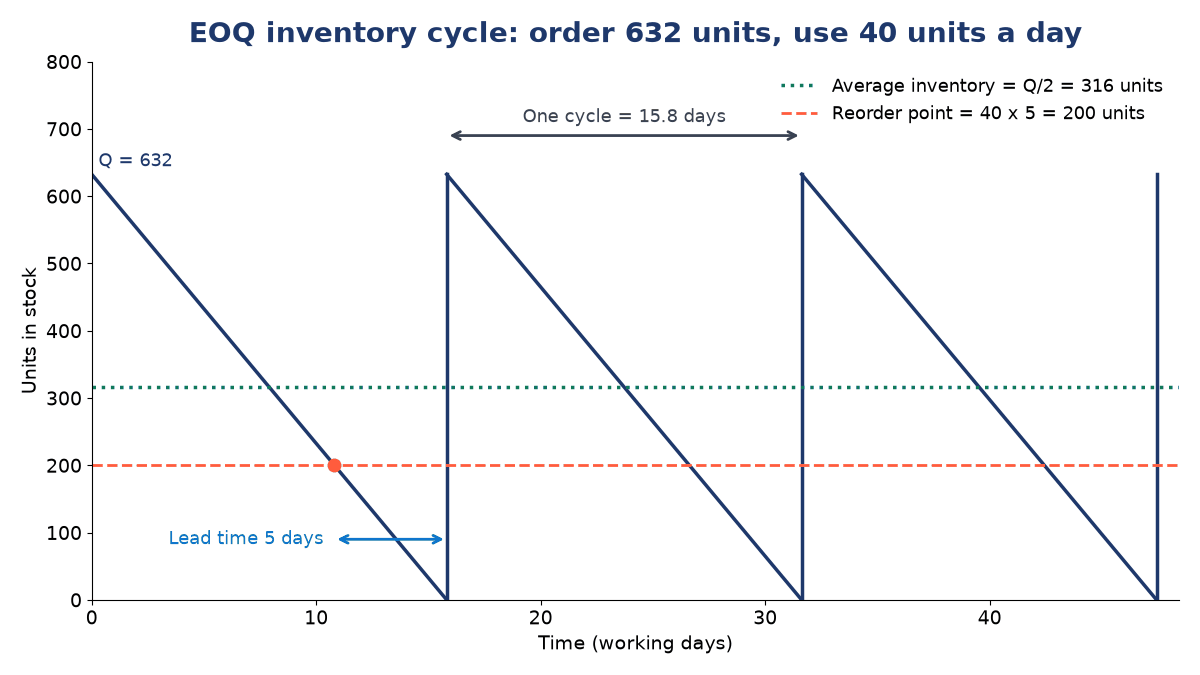
Stock rises to the order quan­tity when a deliv­ery arrives and falls steadily as it is used, which is why aver­age inven­tory is $\displaystyle \frac{EOQ}{2}$. If EOQ is 600 units, aver­age inven­tory is about 300 units. When safety stock is kept, aver­age inven­tory becomes $\displaystyle \frac{EOQ}{2} + \text{safety stock}$.

Assump­tions of the basic EOQ model

• Demand is known and con­stant through­out the year.
• Order­ing cost per order is con­stant, what­ever the order size.
• Hold­ing cost per unit per year is con­stant.
• Pur­chase price is con­stant; no quan­tity dis­counts.
• Lead time is known and con­stant.
• The whole order arrives at once (instan­ta­neous replen­ish­ment).
• No stock-outs are allowed.
• The model deals with a sin­gle item.

These assump­tions keep the model sim­ple; real life is usu­ally more com­pli­cated, so exten­sions exist.

What EOQ does and does not tell

EOQ tells how much to order. It does not tell when to order; that is decided by the reorder point, using lead time and safety stock.

For exam­ple, with EOQ of 400 units and safety stock of 50 units, the firm orders 400 each time but keeps 50 extra as pro­tec­tion. EOQ works best along­side safety stock and reorder plan­ning. It is one tool inside the wider sys­tem of inven­tory man­age­ment, whereas ABC is an item-clas­si­fi­ca­tion tool.

Exten­sions of the basic model

EOQ with quan­tity dis­counts

Sup­pose, in the worked exam­ple, the sup­plier offers a 2% dis­count (price ₹49 instead of ₹50) on orders of 1,000 units or more, and hold­ing cost stays at 10% of price, so $H$ becomes ₹4.90.

EOQ at the dis­counted price is $\displaystyle \sqrt{\frac{2 \times 10{,}000 \times 100}{4.90}} \approx 639$, which is below 1,000, so the low­est valid quan­tity at that price is 1,000. Com­pare total annual cost includ­ing pur­chase cost:

$$TC_{632} = (10{,}000 \times 50) + 3{,}162.28 = \text{ ext{₹}}5{,}03{,}162.28$$

$$\displaystyle TC_{1000} = (10{,}000 \times 49) + \frac{10{,}000}{1{,}000} \times 100 + \frac{1{,}000}{2} \times 4.90 = 4{,}90{,}000 + 1{,}000 + 2{,}450 = \text{ ext{₹}}4{,}93{,}450$$

Order­ing 1,000 units saves ₹9,712.28 a year, so the dis­count should be accepted.

Pro­duc­tion order quan­tity (EPQ)

When items are pro­duced inter­nally and arrive grad­u­ally at pro­duc­tion rate $p$ while being used at rate $d$, the eco­nomic pro­duc­tion quan­tity is $\displaystyle \sqrt{\frac{2DS}{H\left(1 - \frac{d}{p}\right)}}$, where $S$ is set-up cost.

EOQ with planned short­ages

Some mod­els allow lim­ited, planned short­ages (back-orders) when hold­ing cost is high and cus­tomers will wait. With a short­age (back-order) cost $B$ per unit per year, the opti­mal order size is $\displaystyle \sqrt{\frac{2DS}{H}} \times \sqrt{\frac{H + B}{B}}$. As short­age cost becomes very large (tends to infin­ity), the sec­ond fac­tor approaches 1 and the model reduces to the basic no-short­age EOQ. For most under­grad­u­ate exams, the focus remains the no-short­age model.

Advan­tages of EOQ

• Reduces total inven­tory cost by bal­anc­ing order­ing and car­ry­ing costs.
• Improves order­ing deci­sions with a sci­en­tific order size.
• Pre­vents over-order­ing and unnec­es­sary stock accu­mu­la­tion.
• Pre­vents too-fre­quent order­ing and the waste of many small orders.
• Sup­ports inven­tory plan­ning for pur­chase, stores and finance.
• Easy to under­stand and robust to small esti­ma­tion errors.

Lim­i­ta­tions of EOQ

• Demand is rarely con­stant in real life.
• Hold­ing cost may change with inter­est rates, rent and insur­ance.
• Order­ing cost may dif­fer between sup­pli­ers and sit­u­a­tions.
• Lead time may be unsta­ble because of sup­plier delays.
• The basic model ignores short­ages and safety stock.
• The basic model ignores quan­tity dis­counts.
• Costs such as $S$ and $H$ are hard to mea­sure pre­cisely.
• It is less suit­able for depen­dent demand items, which are bet­ter planned with MRP.

EOQ is there­fore a help­ful guide to be used with prac­ti­cal judge­ment.

When and where EOQ is most use­ful

EOQ works best when demand is fairly sta­ble, the item is used reg­u­larly, order­ing and hold­ing costs are known, and short­ages are unde­sir­able. Exam­ples:

• Man­u­fac­tur­ing: steel, screws, pack­ing mate­ri­als, spare parts.
• Retail: note­books, gro­ceries, pack­aged goods.
• Hos­pi­tals: gloves, syringes and med­i­cines with sta­ble demand.

It is use­ful wher­ever stock is ordered reg­u­larly, not only in fac­to­ries.

Key terms

Eco­nomic Order Quan­tity (EOQ)

The order size that min­imises the sum of annual order­ing and car­ry­ing costs.

Annual demand (D)

Total units required or used in a year.

Order­ing cost (S)

Cost of plac­ing and receiv­ing one order.

Hold­ing cost (H)

Cost of car­ry­ing one unit in stock for one year.

Aver­age inven­tory

Half the order quan­tity under steady use, plus any safety stock.

Reorder point

Stock level at which a new order is placed.

Quan­tity dis­count

A lower unit price offered for orders above a stated size.

Eco­nomic pro­duc­tion quan­tity

EOQ adapted for items pro­duced inter­nally and received grad­u­ally.

Com­mon ques­tions

At EOQ, what is the rela­tion­ship between order­ing cost and car­ry­ing cost?

They are equal. In the worked exam­ple both are ₹1,581.14, giv­ing the min­i­mum total of ₹3,162.28.

What hap­pens to EOQ if order­ing cost dou­bles?

EOQ rises by a fac­tor of $\sqrt{2}$, about 41%, not by 100%, because order­ing cost sits inside a square root.

Does EOQ tell when to order?

No. EOQ gives the order size; the reorder point, based on lead time demand and safety stock, gives the tim­ing.

Why is aver­age inven­tory taken as EOQ/2?

Stock falls evenly from the order quan­tity to zero over each cycle, so the aver­age of the high­est and low­est lev­els is half the order quan­tity.

Is pur­chase price included in the basic EOQ for­mula?

No. With a con­stant price it does not affect the choice of order size. It becomes rel­e­vant when quan­tity dis­counts are offered.

What are the main assump­tions of EOQ?

Known and con­stant demand, con­stant order­ing and hold­ing costs, con­stant price, known lead time, instan­ta­neous replen­ish­ment and no short­ages.

Ref­er­ences

1. Har­ris, F. W. (1913) "How Many Parts to Make at Once". Fac­tory, The Mag­a­zine of Man­age­ment, 10(2), 135–136.
2. Steven­son, W. J. Oper­a­tions Man­age­ment. McGraw-Hill Edu­ca­tion.
3. Heizer, J., Ren­der, B. and Mun­son, C. Oper­a­tions Man­age­ment: Sus­tain­abil­ity and Sup­ply Chain Man­age­ment. Pear­son.
4. Pan­neer­sel­vam, R. Pro­duc­tion and Oper­a­tions Man­age­ment. PHI Learn­ing.
5. Chary, S. N. Pro­duc­tion and Oper­a­tions Man­age­ment. McGraw-Hill Edu­ca­tion (India).

Related read­ing

• Inven­tory Con­trol Tech­niques in Oper­a­tions Man­age­ment
• MRP in Oper­a­tions Man­age­ment (Mate­r­ial Require­ments Plan­ning)
• Work Study in Oper­a­tions man­ag­ment