Forecasting is the process of estimating future demand, sales, needs or trends from past data and present conditions, so that a business can plan ahead. A college predicting next year's admissions and a bakery estimating how many cakes it will sell this weekend are both forecasting.
In operations management almost every plan starts with a forecast. It tells a business how much to produce, how many workers are needed, how much raw material to buy and how much stock to keep. A poor forecast leads to overproduction and waste, or to stock-outs and lost customers; a good one lowers cost and uncertainty across the whole organisation.
Meaning and definition
Forecasting is the process of estimating future events, especially demand, for planning and decision-making purposes. A forecast is a statement about the future; it is not a plan or a target. The plan (how much to make) is decided after the forecast (how much customers are likely to buy).
Every forecast has three parts: what is being forecast (units, rupees, hours), for which period (the forecast horizon), and how accurate it is likely to be.
Why forecasting is important
Forecasting supports:
- production planning: deciding output levels;
- inventory control: deciding how much stock to hold and when to reorder;
- manpower planning: hiring, shifts and overtime;
- budgeting: estimating revenue and costs;
- capacity planning: deciding whether to add machines, space or branches;
- reducing shortage and wastage.
Without forecasting, goods may be overproduced, stock may run out, costs may increase and customer demand may not be met.
Types of forecasting by time horizon
Forecasts are commonly grouped by how far ahead they look. Many textbooks add a medium-term category between the two classic types.
1. Short-term forecasting
Covers days, weeks or a few months (usually up to about three months). It is used for daily production, scheduling workers, ordering raw materials and setting job assignments. Example: a restaurant predicts weekend customer demand.
2. Medium-term forecasting
Covers roughly three months to two years. It is used for sales planning, production planning and budgeting, and aggregate planning of workforce and inventory. Example: a garment maker estimates demand for the coming festival and winter seasons.
3. Long-term forecasting
Covers several years. It is used for expansion plans, new product decisions, investment planning, capacity increases and facility location. Example: a school estimates student strength for the next three years before building new classrooms.
| Horizon | Typical period | Used for | Usual methods |
|---|---|---|---|
| Short term | Up to about 3 months | Scheduling, purchasing, staffing | Moving average, exponential smoothing |
| Medium term | 3 months to 2 years | Budgeting, aggregate planning | Trend projection, regression |
| Long term | 2 years and more | Capacity, location, new products | Qualitative methods, regression |
Short-term forecasts are generally more accurate than long-term ones, because fewer things can change in a short period.
Demand patterns
Before choosing a method, look at how past demand behaves. A demand series can contain:
- Level (average): demand fluctuates around a constant mean.
- Trend: a steady rise or fall over time.
- Seasonality: a repeating pattern within a year (ice cream in summer, sweets at Diwali).
- Cycles: longer up-and-down movements linked to the economy.
- Random variation: unexplained noise that no method can predict.
Methods of forecasting
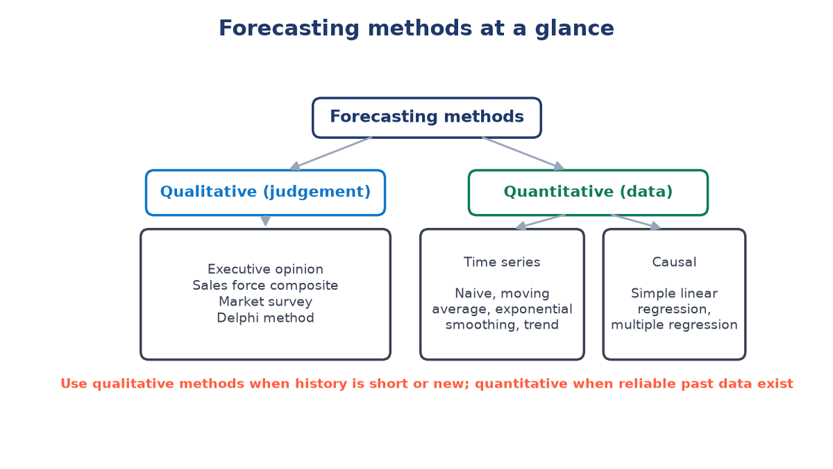
Methods are divided into two broad groups: qualitative and quantitative.
A. Qualitative methods
These rely on judgement, opinion, experience and market knowledge. They are used when past data is limited, for example for a new product, or when conditions are changing fast.
- Jury of executive opinion: senior managers pool their views.
- Sales force composite: each salesperson estimates sales in their territory, and the estimates are added up.
- Market survey (consumer survey): customers are asked about their buying intentions.
- Delphi method: a panel of experts answers questionnaires in several anonymous rounds, with feedback between rounds, until their views converge.
- Expert opinion: specialists outside the firm are consulted.
Example: a company asks experts whether a new course will have enough demand.
B. Quantitative methods
These use numerical data and mathematical techniques. They are used when reliable past data is available.
Time series methods assume that the future will follow the pattern of the past:
- Naive method: next period's forecast equals this period's actual demand.
- Simple moving average: the average of the last periods.
- Weighted moving average: recent periods get larger weights.
- Exponential smoothing: the new forecast is the old forecast plus a fraction of the last error.
- Trend projection: a straight line fitted to past data by least squares and extended forward.
Causal (associative) methods link demand to other variables, such as price, advertising or population, usually through linear regression.
Example: a store studies the last 12 months' sales to estimate next month's sales.
Key formulas
Simple moving average over periods:
Weighted moving average, with weights that add up to 1:
Simple exponential smoothing, with smoothing constant between 0 and 1:
Mean absolute deviation (MAD), a common accuracy measure:
Here is actual demand and is the forecast for period . A larger makes the forecast respond faster to recent changes; a smaller gives a smoother forecast.
Worked example: moving average and exponential smoothing
Suppose a bakery recorded the following monthly cake sales and wants a forecast for Month 9.
| Month | 1 | 2 | 3 | 4 | 5 | 6 | 7 | 8 |
|---|---|---|---|---|---|---|---|---|
| Actual demand (cakes) | 120 | 130 | 125 | 140 | 150 | 145 | 160 | 165 |
Step 1: three-month moving average
The first forecast possible is for Month 4, using Months 1 to 3:
Moving the window forward one month at a time:
The moving average forecast for Month 9 is about 157 cakes.
Step 2: weighted moving average
If the bakery gives weights of 0.5, 0.3 and 0.2 to the latest, second-latest and third-latest months:
The weighted forecast (about 160 cakes) is higher because it leans more on the rising recent months.
Step 3: exponential smoothing with alpha = 0.3
Assume the forecast for Month 1 was 120. Then:
The exponential smoothing forecast for Month 9 is about 151 cakes.
Step 4: compare accuracy using MAD (Months 4 to 8)
| Month | Actual | 3-month MA | Absolute error (MA) | Exp. smoothing | Absolute error (ES) |
|---|---|---|---|---|---|
| 4 | 140 | 125.00 | 15.00 | 123.60 | 16.40 |
| 5 | 150 | 131.67 | 18.33 | 128.52 | 21.48 |
| 6 | 145 | 138.33 | 6.67 | 134.96 | 10.04 |
| 7 | 160 | 145.00 | 15.00 | 137.97 | 22.03 |
| 8 | 165 | 151.67 | 13.33 | 144.58 | 20.42 |
| Total | 68.33 | 90.37 | |||
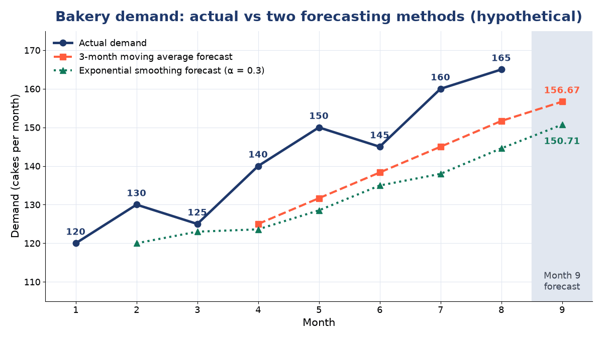
Interpretation: the moving average has the lower MAD, so it was more accurate for this data. Both methods lag behind a rising trend, and exponential smoothing with a small of 0.3 lags the most. For data with a clear trend, a larger or a trend-adjusted method would usually do better.
Steps in the forecasting process
- Decide the purpose of the forecast and how it will be used.
- Select the items to be forecast and the time horizon.
- Collect and clean the relevant data.
- Examine the data for level, trend and seasonal patterns.
- Select a suitable forecasting method.
- Prepare the forecast.
- Monitor accuracy by comparing forecasts with actual results, and revise the method when errors grow.
Qualities of a good forecast
A good forecast should be:
- simple and easy to understand;
- timely, available before decisions must be made;
- reasonably accurate, with its likely error stated;
- economical, costing less than the benefit it gives;
- reliable and consistent over time;
- expressed in meaningful units (cakes, hours, rupees).
Factors affecting forecasting
- market demand and customer preferences;
- competition and competitors' pricing;
- seasonal changes and festivals;
- government policy and taxes;
- general economic conditions;
- technology changes;
- the firm's own promotions and prices.
A real-life illustration: an ice cream shop
In summer, demand for ice cream is high; in the rainy season it is lower. The shop forecasts demand for each season and uses that forecast to decide how much stock to keep, how many workers are needed and how much milk and sugar to buy. Recognising the seasonal pattern is what makes the forecast useful.
Advantages and limitations
| Advantages | Limitations |
|---|---|
| Better planning of production, stock and staff | The future is uncertain; a forecast may be wrong |
| Better use of resources and lower cost | Accuracy depends on the quality of data |
| Improved customer satisfaction through fewer stock-outs | Sudden market changes reduce accuracy |
| Supports decision-making and reduces uncertainty | Qualitative methods can be biased |
| Helps coordinate departments around one estimate | Long-range forecasts are less reliable than short-range ones |
Forecasting is helpful, but it is never perfect. Good practice is to state the expected error and to keep monitoring.
Exam answer formats
5-mark answer. Forecasting is the process of estimating future demand or future events for planning purposes. It is important in operations management because it helps in production planning, inventory control, manpower planning and budgeting. Forecasts may be short-term, medium-term or long-term. The main methods are qualitative (such as the Delphi method and market surveys) and quantitative (such as moving averages and exponential smoothing). Good forecasting reduces uncertainty and improves decision-making.
2-mark answer. Forecasting is the process of predicting future demand or future events for planning and decision-making.
Memory line. Forecasting means looking ahead so that planning is better.
Key terms
- Forecast
- An estimate of a future value, such as demand, for a stated period.
- Forecast horizon
- The length of time into the future that a forecast covers.
- Time series
- A set of observations recorded at regular time intervals.
- Moving average
- The average of the most recent periods, used as the next forecast.
- Exponential smoothing
- A method that updates the last forecast by a fraction of the last error.
- Smoothing constant
- The weight , between 0 and 1, given to the most recent error.
- Delphi method
- A qualitative method using anonymous, repeated rounds of expert opinion.
- Mean absolute deviation
- The average of the absolute forecast errors, used to measure accuracy.
- Seasonality
- A demand pattern that repeats at regular intervals within a year.
Common questions
What is the difference between qualitative and quantitative forecasting?
Qualitative methods rely on judgement and opinion and are used when data is scarce, such as for a new product. Quantitative methods use past numerical data and mathematical models and are used when reliable history exists.
Which value of alpha should be used in exponential smoothing?
A higher (for example 0.5 or more) reacts quickly to recent changes but also to random noise. A lower (0.1 to 0.3) gives a smoother, more stable forecast. The best value is usually the one that gives the lowest error, such as MAD, on past data.
Why do moving averages lag behind a trend?
A moving average gives equal weight to older periods, so when demand is rising steadily the average is always pulled down by the older, lower values. Weighted averages and trend methods reduce this lag.
What is the difference between a forecast and a plan?
A forecast estimates what customers are likely to demand. A plan decides what the firm will actually do, such as how much to produce, taking the forecast, capacity and costs into account.
How is forecast accuracy measured?
By comparing forecasts with actual results. Common measures are mean absolute deviation (MAD), mean squared error (MSE) and mean absolute percentage error (MAPE). A lower value means a more accurate method.
References
- Heizer, J., Render, B. and Munson, C. Operations Management: Sustainability and Supply Chain Management. Pearson.
- Stevenson, W. J. Operations Management. McGraw-Hill Education.
- Chase, R. B. and Jacobs, F. R. Operations and Supply Chain Management. McGraw-Hill Education.
- Brown, R. G. (1959) Statistical Forecasting for Inventory Control. McGraw-Hill.
- Chary, S. N. Production and Operations Management. McGraw-Hill Education (India).